Lab 8: Drift Stunt

Overview

The objective of Lab 8 was to execute a high-speed robotic stunt, demonstrating the integration of sensing, control, and actuation pipelines. I chose to implement the “Drift” stunt, which required the robot to accelerate toward a wall, detect proximity, perform a 180° spin, and return in the opposite direction. Although my initial implementation used an open-loop timing-based spin, I adapted the control structure from my Lab 6 PID yaw controller to simulate closed-loop behavior. The robot used the ToF sensor to trigger the spin at a fixed threshold and followed a time-calibrated turn to emulate yaw setpoint convergence.

Control Logic and Integration

Open-Loop Drift Stunt

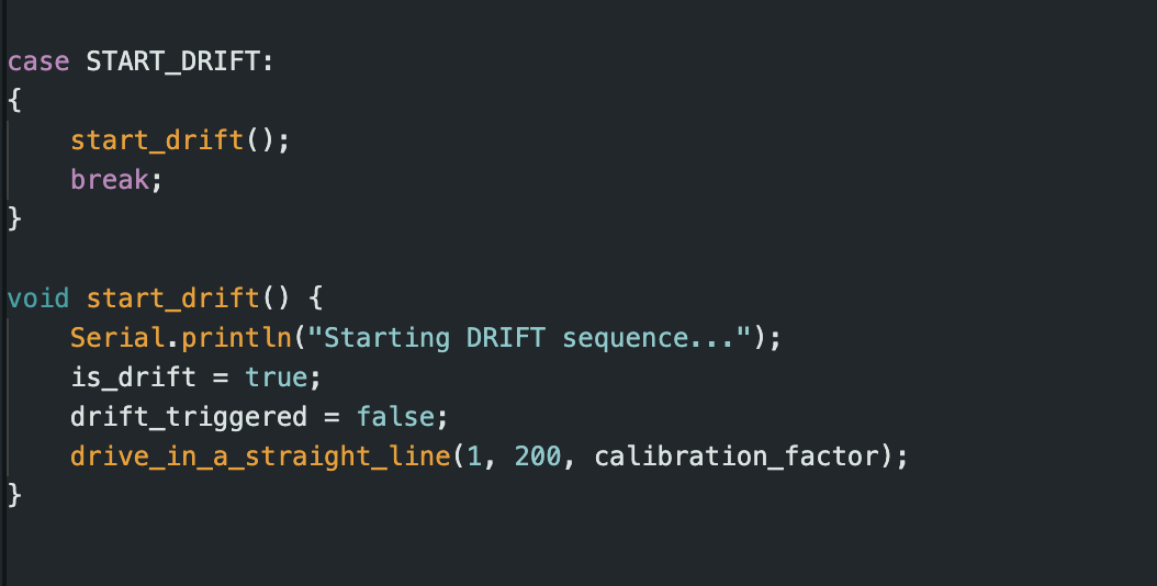
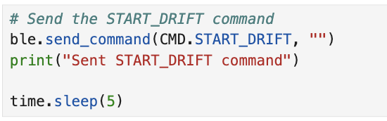
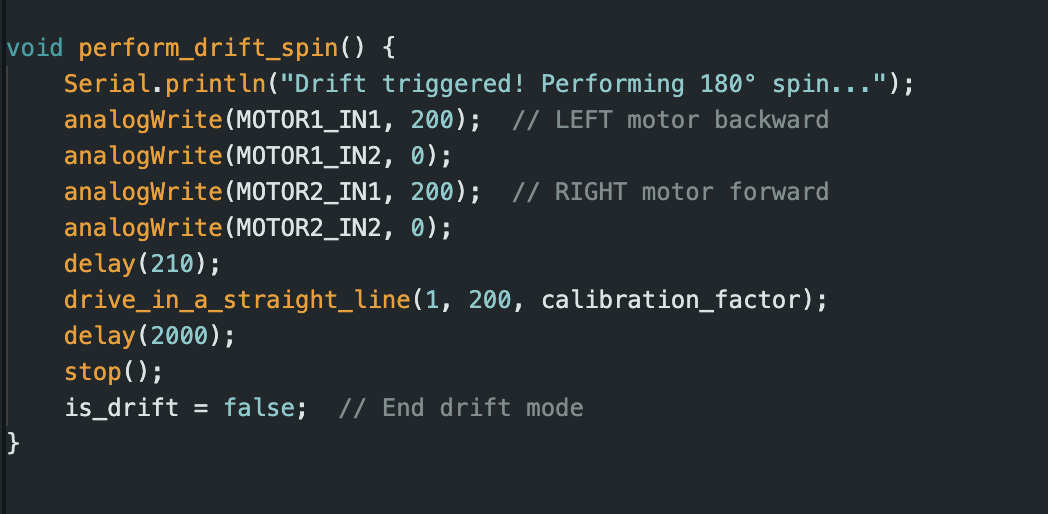
I began implementing the drift stunt using a simple open-loop strategy. I added a custom BLE command, START_DRIFT, that triggered the robot to drive forward at high PWM. Once the ToF sensor measured a distance below a threshold of 914 mm (roughly 3 tiles from the wall), the robot executed a timed in-place spin. I achieved this by driving one motor forward and the other in reverse for a calibrated delay of approximately 210–250 ms — enough to rotate the robot close to 180°.

The spin logic was implemented in my perform_drift_spin() function, where I set the left motor to run backward and the right motor forward. After the spin, I commanded the robot to continue driving straight for a fixed amount of time before stopping using a stop() call. This approach made the stunt fully open-loop but reliable and repeatable, as it relied only on timing and a single ToF threshold trigger.

To manage this sequence cleanly, I introduced two key state flags in my code:

• is_drift – A boolean flag that indicated when the robot was in drift mode after the START_DRIFT command was received.
• drift_triggered – Another flag that prevented the robot from re-triggering the spin logic multiple times after the initial threshold crossing.

I checked these flags inside the loop() function while connected to BLE, which helped me modularize the drift behavior and avoid unwanted repeated spins.

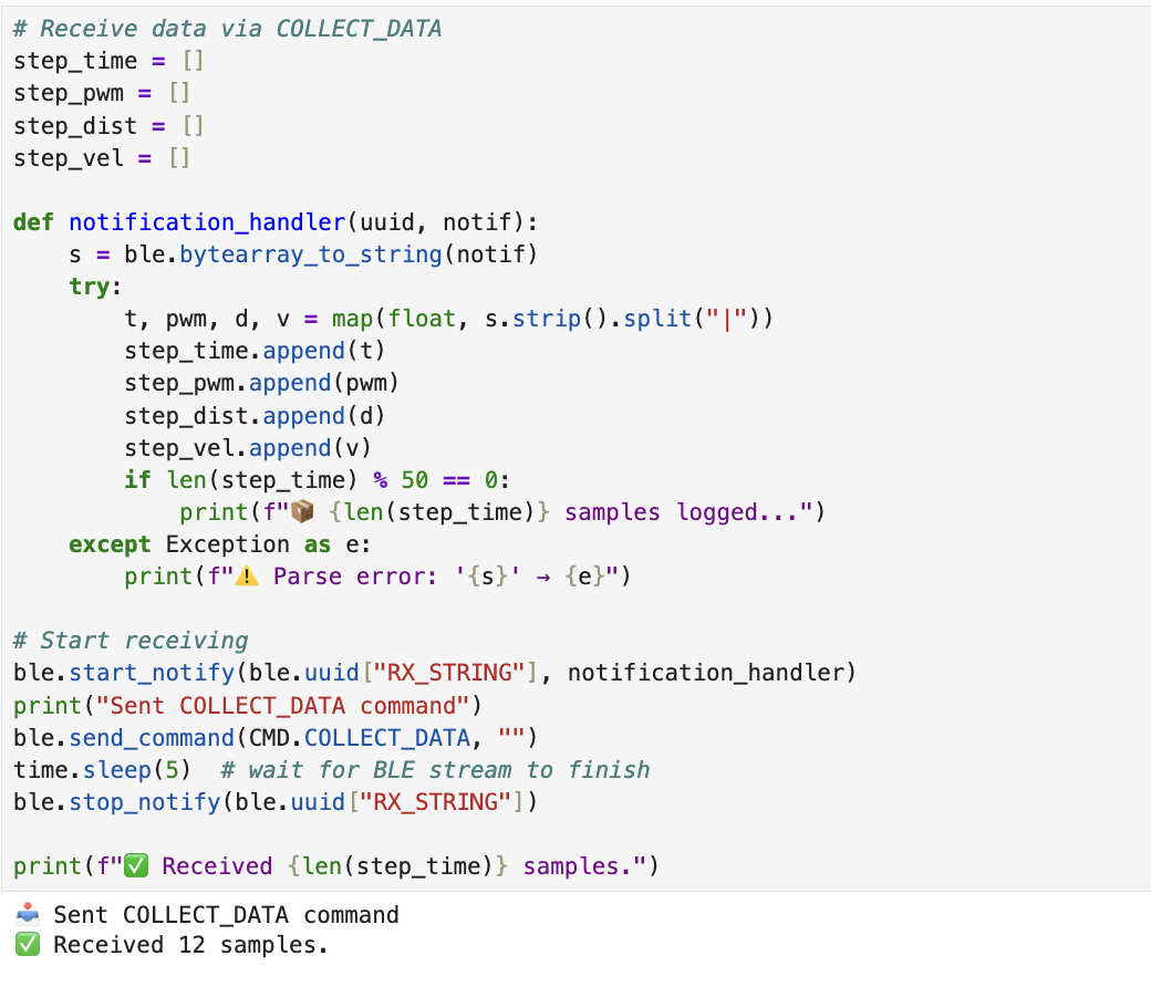
During the drift, I logged time, PWM values, and ToF distances into arrays using log_drift_data(). This data could then be retrieved using my COLLECT_DATA BLE command, just like in previous labs. I reused the same Python notification handler to receive the logs and visualize the data for debugging and validation.

Closed-Loop Drift Stunt

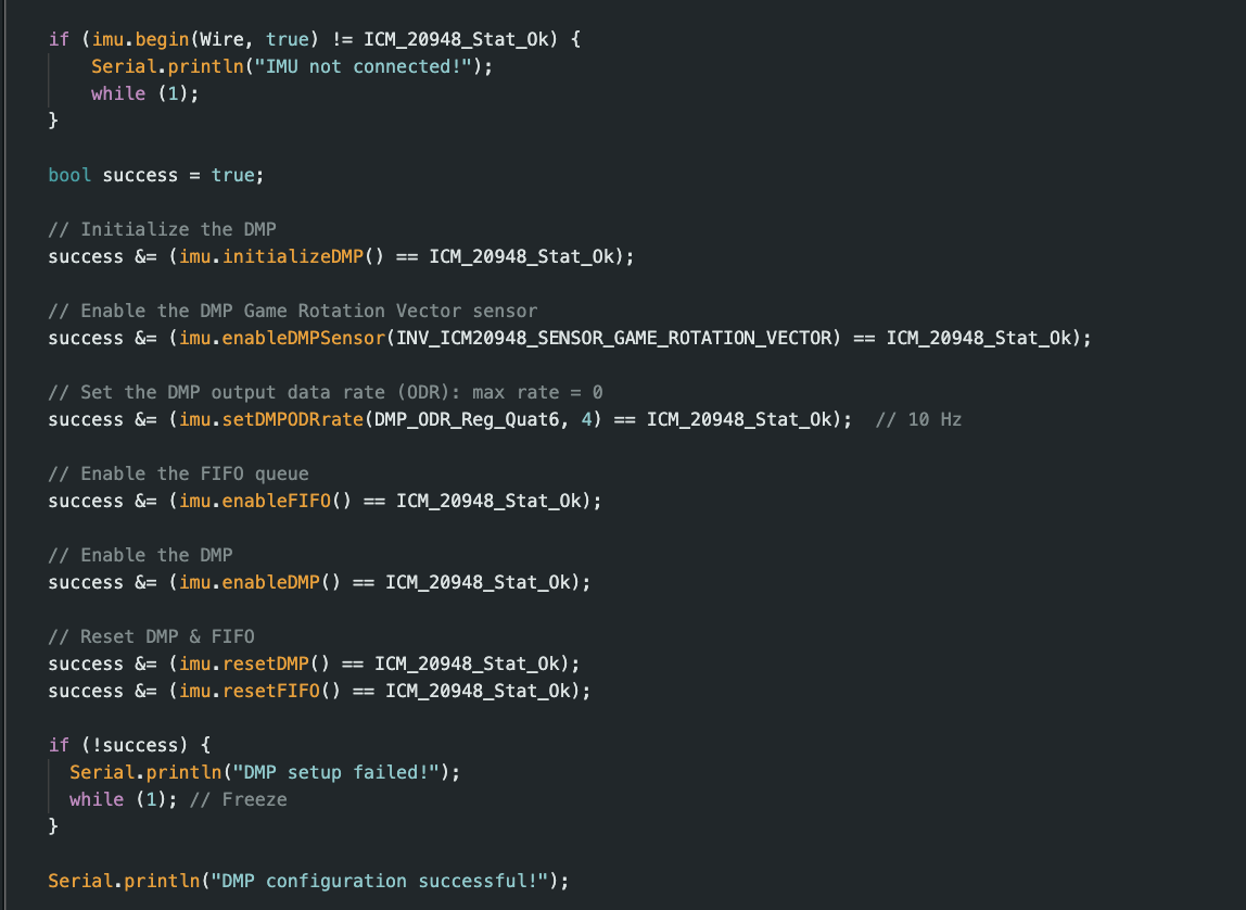
While my open-loop implementation was repeatable and functional, it lacked adaptability to changes in surface friction, battery level, or wheel slippage. To improve it and bring the stunt closer to the lab's closed-loop expectations, I leveraged my Lab 6 PID yaw controller, which was built around the IMU's onboard Digital Motion Processor (DMP).

I configured my IMU to output Euler angles. The record_dmp_data() function then gave me stable high-rate yaw readings that I could use as feedback for angular control.

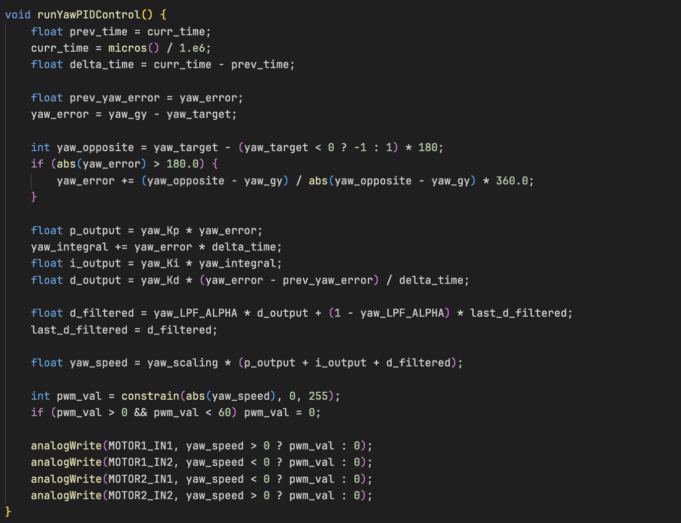
For the closed-loop version of the drift, I replaced the fixed spin delay with a feedback loop that continuously check the yaw, compute the yaw error relative to a 180° setpoint, and apply a PID controller to update the motor commands until the yaw error converges. This structure mirrors my run_yaw_pid_sequence() from Lab 6, where I achieved smooth heading correction using tuned PID gains.

BLE Command Structure & Data Logging

For control and debugging, I continued to build on the BLE command infrastructure I developed in earlier labs. I added a new command called START_DRIFT, which initiated the open-loop stunt sequence when received. This command set the is_drift flag to true and started the robot’s forward motion. The main loop() then continuously checked whether the ToF sensor reading dropped below the threshold, and if so, triggered the perform_drift_spin() function.

To verify behavior and analyze performance after each run, I implemented a logging system using arrays to store time, PWM value, and ToF distance. I reused my log_drift_data() function to collect this data, and created a COLLECT_DATA BLE command that streamed the log back to my Python script via the same notification handler I used in Labs 5 and 6.

This allowed me to plot the robot's approach to the wall and validate that the trigger point occurred around the expected 914 mm mark. It also made it easy to tune the spin delay value by correlating ToF readings with the rotation behavior captured in the logs.

Results & Analysis

After tuning the spin delay and forward PWM values, I was able to reliably trigger a 180° drift stunt near the wall. The robot would approach the wall at high speed, spin in place, and drive away cleanly.

I also captured a blooper moment where the robot turned too early and ended up drifting off to the side. These types of failures typically occurred when surface friction or wheel slip caused the robot to rotate more or less than expected — a natural limitation of open-loop control.

Although I implemented BLE-based logging and streamed back ToF and PWM values during runs, I ultimately decided not to include plots in this write-up. The raw logs were consistent with expectations, but the videos themselves did a better job demonstrating failure and success modes.

Conclusion

This lab brought together nearly every system I built throughout the semester — from BLE command handling and ToF sensing to motor control and PID feedback logic. I started with a simple open-loop approach to executing the drift stunt and was able to reliably perform a 180° spin near a wall using timed motor commands and sensor-triggered logic.

To align with the closed-loop goals of the course, I drew on my Lab 6 PID yaw controller and integrated the IMU’s DMP-based yaw feedback pipeline into the stunt logic.

[1] Huge thanks to Stephan Wagner (2024) for his inspiration and helpful documentation throughout this process.