Lab 12: Path Planning and Execution

Objective

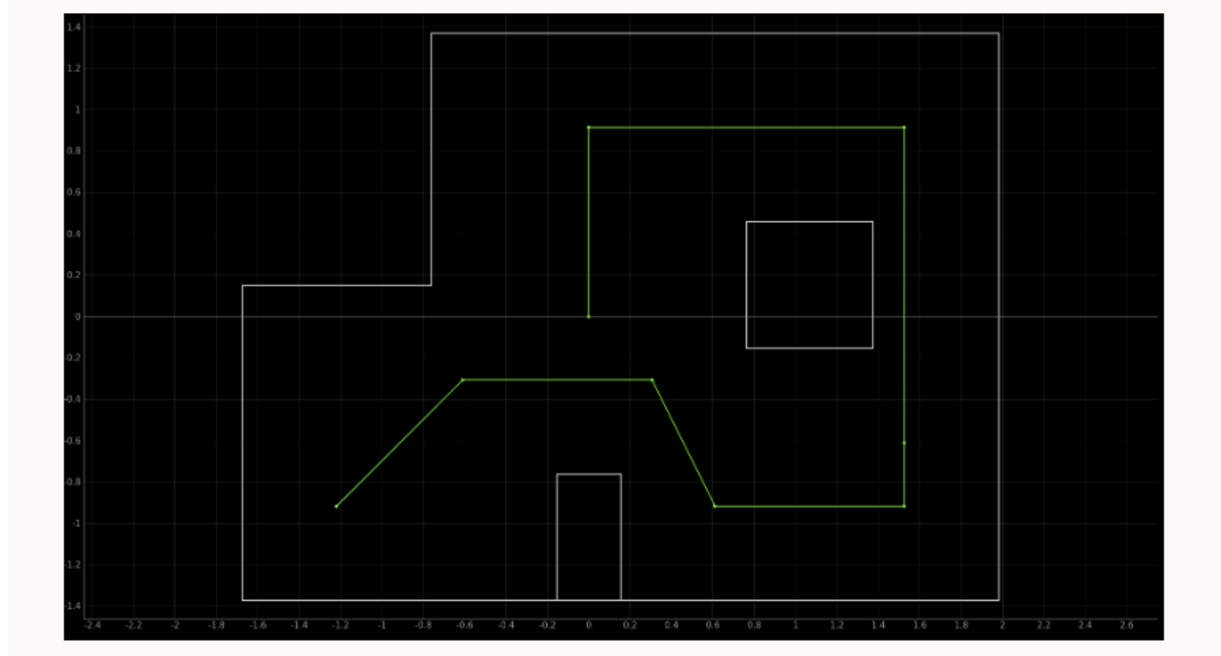
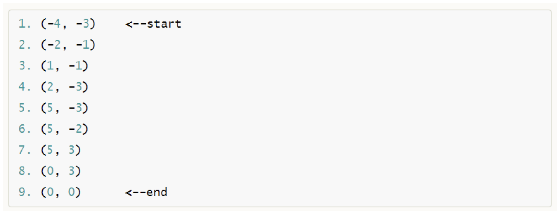
So far we have worked and implemented open and closed loop control on our robot, performed an amazing stunt in lab 6. Now this lab served as the last lab of the semester, the final step is now have the robot navigate through a set of waypoints in a boxed environment as quickly and accurately as possible.

My original goal for Lab 12 was to implement a closed-loop motion planning system that could guide the robot along a predefined map using real-time localization and feedback. I planned to use yaw measurements from the IMU and a PID controller to perform accurate rotations, allowing the robot to align itself before driving forward to each target position.

However, despite multiple attempts, I struggled to get the IMU-based yaw estimates and PID orientation control to work reliably. The robot’s rotation was inconsistent, and I wasn’t able to achieve stable heading correction. Because of these issues — and with the deadline approaching — I made the decision to pivot to an open-loop strategy.

Instead of relying on feedback, I hardcoded a sequence of timed drive and turn commands. This allowed the robot to approximately follow the intended path on the map. Although the final approach lacked precision, it demonstrated the basic planning logic and served as a functional solution given the time constraints and hardware limitations.

Implementation Overview

I began the lab by building on work I had developed in previous labs. My initial plan was to use the IMU to track yaw and perform PID-based orientation control. I reused the same setup from Lab 6 to initialize the DMP on the ICM-20948 and read quaternion-based yaw angles. I also reimplemented my PID control function to handle yaw corrections during in-place turns.

Unfortunately, the yaw data proved too noisy and inconsistent, even after resetting the DMP and fine-tuning my gains. Because the localization step was unreliable, I commented out the PID logic and moved forward with an open-loop navigation strategy.

The video above shows the failed attempt at closed-loop rotation control — the robot spins inconsistently and fails to settle at the intended angles. This confirmed our decision to abandon closed-loop localization due to time constraints.

To enable this, I created three custom BLE commands — DRIVE_FORWARD, TURN_LEFT, and TURN_RIGHT — each triggering a simple motor routine with a fixed delay. I also implemented a higher-level command called RUN_MISSION that executed the entire path using a hardcoded sequence of forward drives and left/right turns.

This allowed the robot to traverse a simplified map route without relying on sensors or localization. While the robot’s motion was imprecise, the approach worked well enough to demonstrate basic path execution logic and recover functionality under a tight deadline.

Execution Behavior

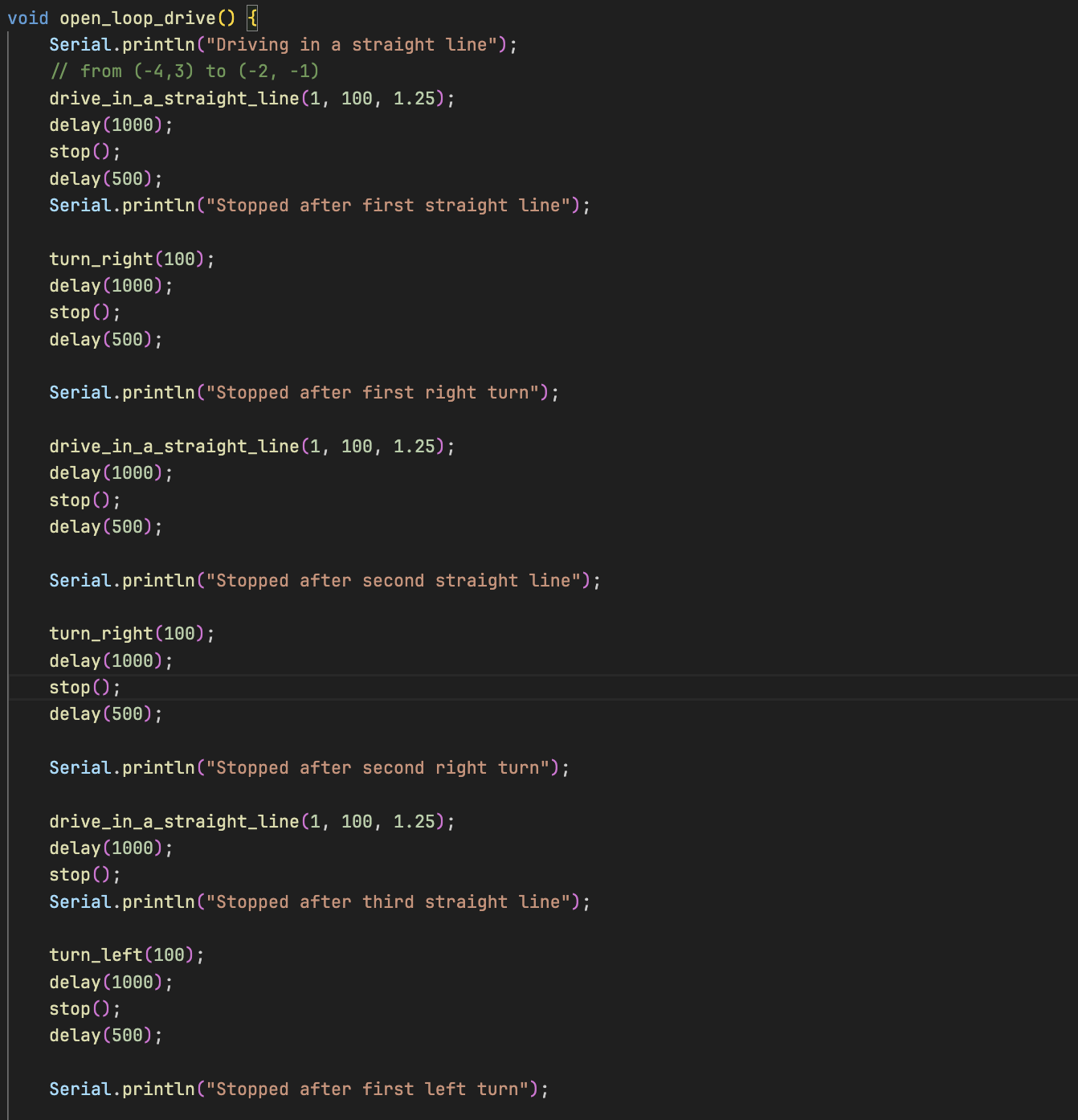
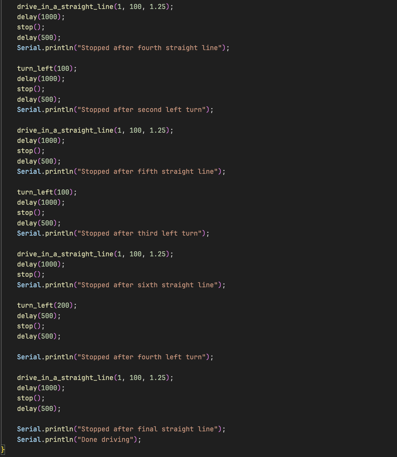
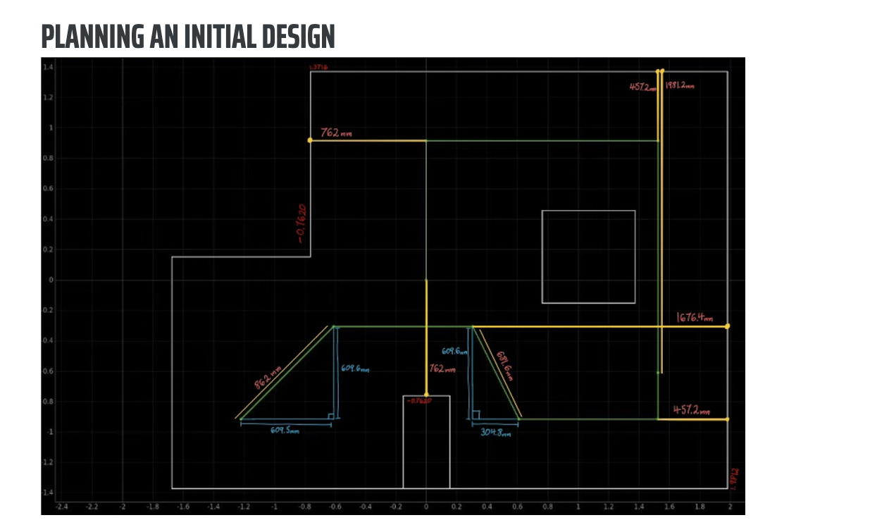
I implemented the mission path in a function called open_loop_drive(), which sequenced together timed drive and turn actions based purely on PWM values and delay(). To figure out how far to travel and when to turn, I referenced a brilliant diagram from Mikayla Lahr's Lab 12 report — her measured path distances and angles came in clutch. I used her diagram to estimate both straight-line distances (in milliseconds) and turn durations for 90° turns.

I triggered the sequence with a RUN_MISSION BLE command, which began a series of forward motions and 90° turns using only analogWrite() and delay(). I empirically tuned the motor durations based on the expected lengths shown in the plan — for example, I set 1000ms of forward drive for a ~0.6m segment, and 1000ms for turns. Between each move, I added short delay(500) pauses to allow the robot to settle before the next step.

The robot followed the path reasonably well despite lacking any feedback. Because this was open-loop, drift did occur — especially after several turns — but overall, the robot ended near the expected goal. It completed all forward segments and the correct number of left and right turns without stalling or crashing. This strategy saved our lab despite localization issues with the IMU.

Conclusion

Lab 12 was a humbling but rewarding experience that reminded me of the importance of flexibility in engineering. My initial plan was to close the loop on localization and motion control using yaw data from the IMU and PID-based corrections. I had reused my DMP setup and PID logic from Lab 6, but despite multiple attempts at tuning and resets, the IMU yaw remained unreliable, making stable orientation control nearly impossible.

Rather than let that setback stall my progress, I shifted toward a fully open-loop implementation. I hardcoded drive and turn sequences using BLE commands and fixed delays. I tuned these by hand and stitched them into a RUN_MISSION routine that approximated the desired path. While this approach lacked precision, it got the job done and salvaged my ability to demonstrate core path planning concepts under pressure.

I want to acknowledge Akinfolami Akin-Alamu for being a great teammate and collaborator throughout the semester. I also drew inspiration from Mikayla Lahr’s Lab 12 report, whose distance and timing map played a critical role in helping me tune my mission routine.

At the end of the day, I learned that engineering isn’t always about getting it perfect — sometimes it’s about making something work when it matters most.