Lab 11: Real-World Localization
Objective
In this lab, my goal was to perform real-world localization using the Bayes Filter’s update step — relying solely on sensor measurements from the ToF sensor. Unlike previous labs, here I focused entirely on the correction step. I placed the robot at known map locations, performed a 360° sensor sweep, and used that observation to infer the robot’s position on a grid map.
I had the robot perform a full in-place rotation while collecting 18 sensor readings — one every 20 degrees. I then compared these ToF measurements against expected map readings and used them to update the belief distribution over (x, y, θ) poses.
Implementation Overview
I extended my RealRobot class to support a 360° observation loop. The robot rotated slowly in place, capturing 18 evenly spaced ToF measurements.
I used these readings to update the belief over the robot’s pose on a discretized map using only the Bayes Filter’s update step.
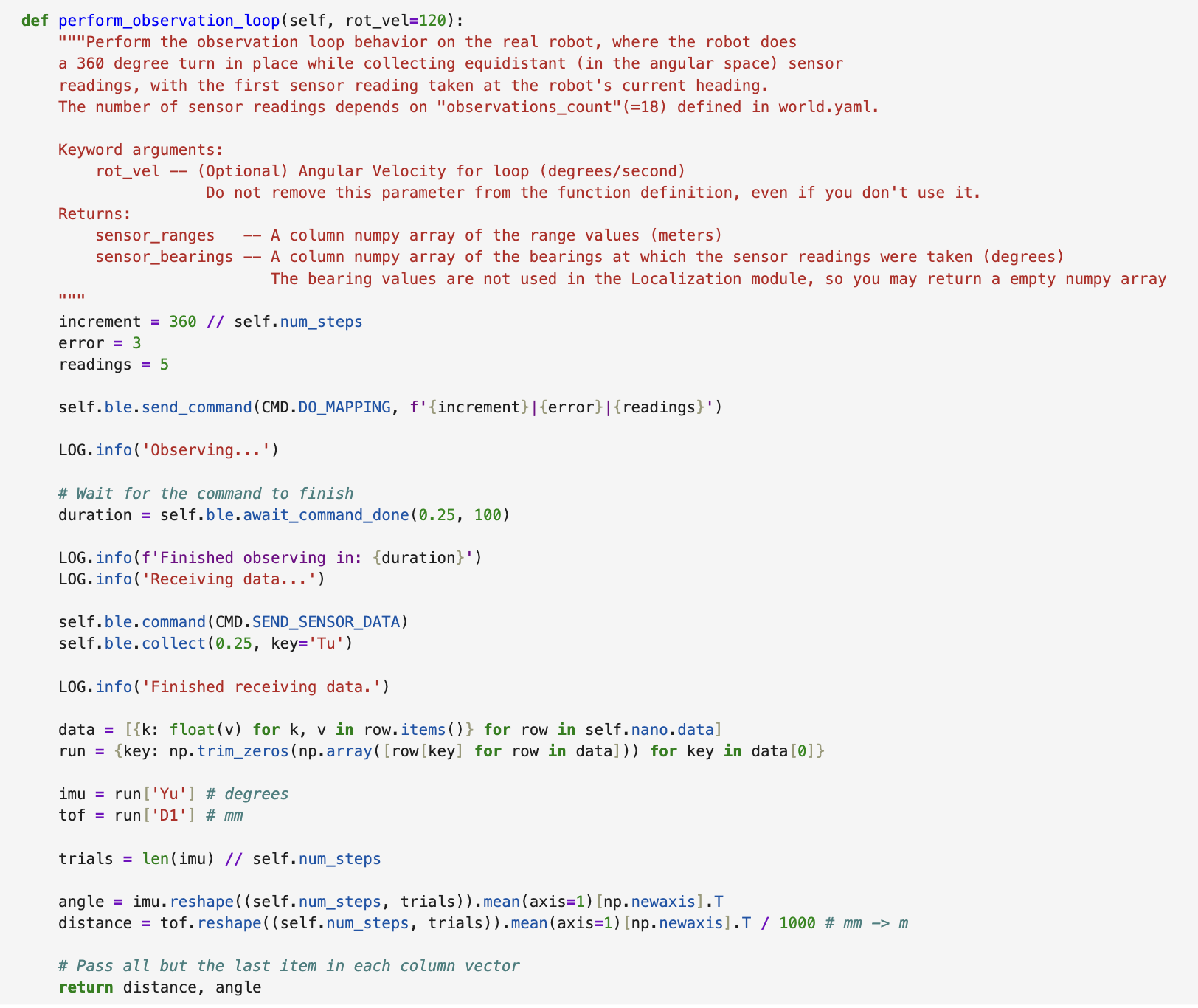
I implemented a new method called perform_observation_loop(), which sent a DO_MAPPING command over BLE to start the 360° scan.
After waiting for the scan to complete, I reshaped and averaged the IMU (yaw) and ToF data into two stable column vectors — one for distances in meters and one for angles in degrees.
These vectors were then passed into the Bayes Filter’s update function.
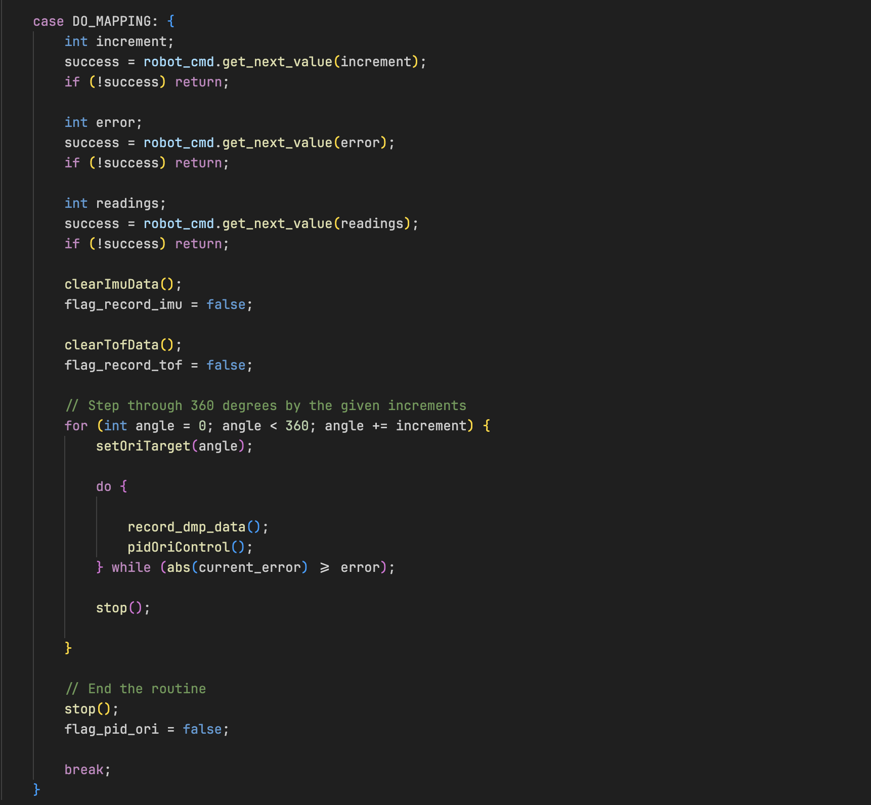
I reused the DO_MAPPING command I had already implemented in lab 10, since it was reliable for triggering 360° scans and collecting sensor values.
I triggered the command via BLE using the same notification handler as previous labs.
Observation Loop Behavior
I wrote the observation loop in perform_observation_loop() inside the RealRobot class.
The robot rotated in place while recording yaw and ToF data every 20°, for a total of 18 observations.
I passed three parameters to the robot:
angular increment (20°), acceptable yaw error (3°), and number of ToF readings per angle (5). I bundled these into a string and sent them using
ble.send_command(CMD.DO_MAPPING, ...). Once the robot completed its turn, I requested the recorded data using CMD.SEND_SENSOR_DATA.
Data Retrieval
After retrieving the data, I reshaped the readings using NumPy and averaged them across repeated trials to reduce noise.
 imu = run['Yu'] # yaw in degrees
 tof = run['D1'] # distance in mm
 angle = imu.reshape((self.num_steps, trials)).mean(axis=1)[np.newaxis].T
 distance = tof.reshape((self.num_steps, trials)).mean(axis=1)[np.newaxis].T / 1000 # convert mm to meters
This gave me two output vectors: sensor_ranges (distances in meters) and sensor_bearings (yaw angles).
I then used sensor_ranges in the Bayes Filter to perform the update.
Evaluation at Test Poses
I tested localization at the four given grid positions: (-3, -2), (0, 3), (5, -3), and (5, 3). At each pose, I triggered a 360° scan and passed the resulting observations into the Bayes Filter. I then visualized the updated belief distribution to evaluate localization accuracy.
.png)
.png)
.png)
.png)
Observations
At (0, 3), I observed a sharply peaked belief centered exactly at the correct pose — the robot localized confidently thanks to clear nearby features. At (5, -3), the belief was slightly more spread out, suggesting some ambiguity due to environmental symmetry. When testing at (-3, -2), I saw a tight and confident belief peak, likely due to unique geometry and distinct scan matches. At (5, 3), the belief was offset slightly, but still concentrated in the right quadrant — showing the robot could localize fairly well even in more ambiguous regions.
Conclusion
This lab showed me that the update step of the Bayes Filter alone is powerful enough to localize a robot using just ToF sensor readings. Even without odometry, I was able to accurately estimate the robot’s pose in a known map using real-world data.
The sensor model worked well at most test locations, and belief distributions were consistently centered near the true pose. Areas with strong geometric features led to more accurate and confident localization, while more symmetric or open spaces introduced some uncertainty. Overall, I found this lab to be a great hands-on example of probabilistic localization in action.
[1] I want to thank Stephan Wagner for documenting his workflow in such a clear and structured way — his guide helped me debug and structure my implementation.